
B-Trees: Why Every Database Uses Them
Understanding the data structure that makes databases fast on disk

Your database has 10 million user records. You query for one user by ID. The database returns the result in 3 milliseconds. How?
If the database scanned all 10 million records sequentially, it would take seconds, maybe minutes. But databases don’t scan. They use an index—and that index is almost certainly a B-Tree.
Every major database system uses B-Trees: MySQL InnoDB, PostgreSQL, SQLite, MongoDB’s WiredTiger storage engine, Oracle Database, Microsoft SQL Server. It’s not a coincidence. B-Trees solve a fundamental problem: how to efficiently find data on disk when disk access is thousands of times slower than memory access.
This is the story of why binary search trees fail on disk, how B-Trees fix that problem, and why after 50+ years, we’re still using them.
The Problem: Binary Search Trees on Disk
Let’s start with what doesn’t work: binary search trees (BSTs) on disk.
In memory, binary search trees are excellent. Each node stores one key and has two children (left and right). Keys in the left subtree are smaller, keys in the right subtree are larger. Finding a key takes O(log₂ n) comparisons.
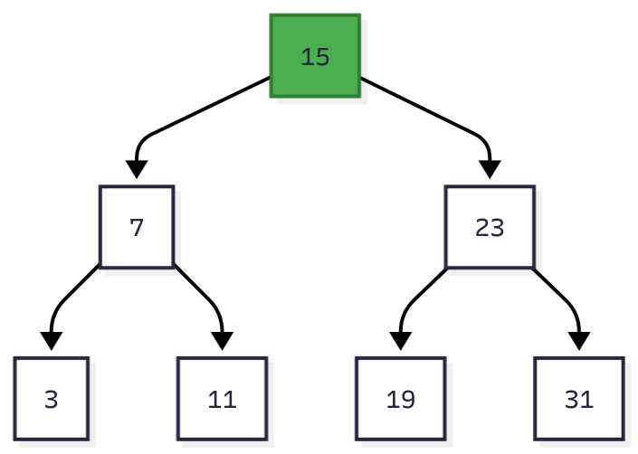
Figure 1: Binary search tree with 7 nodes. Finding key 11 takes 3 comparisons: 15 → 7 → 11.
For 1 million records, a balanced BST has height log₂(1,000,000) ≈ 20. That’s 20 comparisons to find any record.
In memory, this is fast. Each comparison is a pointer dereference (~0.0001 milliseconds on modern CPUs). Total lookup: 0.002 ms.
On disk, this is catastrophic. Here’s why:
Disk I/O is Expensive
The smallest unit of disk access is a block (typically 4 KB to 16 KB). To read a single byte from disk, you must read the entire block containing it.
Disk access times:
Disk is 100-100,000x slower than RAM.
The Binary Tree Disaster
With a BST on disk, each node is stored in a separate disk block. Traversing from parent to child requires a disk seek.
For 1 million records:
Height: 20 nodes
Disk seeks: 20
Time on HDD: 20 × 10 ms = 200 milliseconds
Time on SSD: 20 × 0.1 ms = 2 milliseconds
That’s acceptable for SSDs, but terrible for HDDs. And it gets worse as the tree grows.
For 1 billion records:
Height: 30 nodes
Time on HDD: 30 × 10 ms = 300 milliseconds
Time on SSD: 30 × 0.1 ms = 3 milliseconds
The fundamental problem: BST fanout is too low (only 2 children per node). We need more children per node to reduce tree height.
Why Not Just Balance the Tree?
You might think: “Just keep the tree balanced!” Red-black trees and AVL trees do this.
The problem isn’t just tree height—it’s maintenance cost. Balancing requires rotating nodes and updating pointers. In memory, this is cheap (a few pointer writes). On disk, it’s expensive:
Read the node from disk (4 KB block)
Modify the node in memory
Write the modified node back to disk (4 KB block)
Update parent pointers (more disk I/O)
For a tree with frequent inserts and deletes, constant rebalancing kills performance. We need a data structure that:
Has high fanout (many children per node) → reduces height
Requires infrequent rebalancing → reduces I/O overhead
That data structure is the B-Tree.
What is a B-Tree?
A B-Tree is a self-balancing tree optimized for disk access. Instead of 2 children per node (binary tree), a B-Tree node has hundreds or thousands of children.
Key idea: Each B-Tree node fits in one disk block (4 KB to 16 KB). Since we must read an entire block anyway, pack as many keys as possible into it.
B-Tree Structure
A B-Tree node stores:
N keys (sorted)
N + 1 pointers to child nodes
Each key acts as a separator: keys in child[i] are less than key[i], keys in child[i+1] are greater than or equal to key[i].
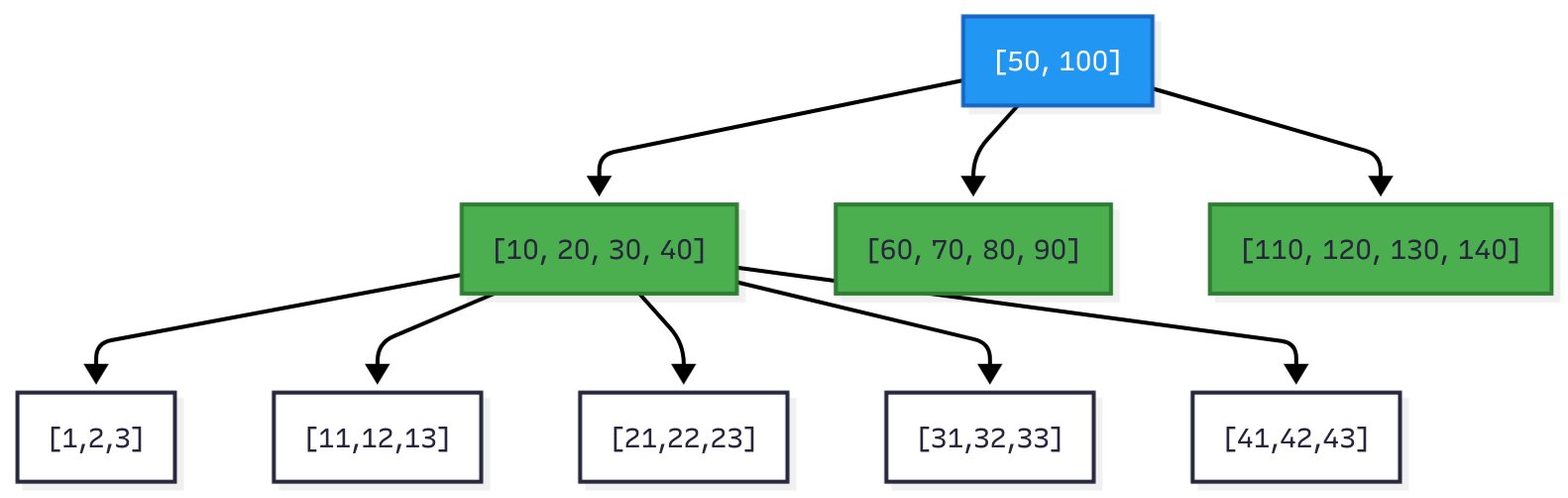
Figure 2: B-Tree with fanout ~100. Root has 2 keys and 3 children. Internal nodes have 4 keys and 5 children. Leaf nodes contain actual data.
B-Tree Hierarchy
B-Trees have three types of nodes:
Root node: The top of the tree. There’s always exactly one root.
Internal nodes: Middle layers that guide searches. They store separator keys and pointers, but no actual data.
Leaf nodes: Bottom layer containing the actual data (key-value pairs). All leaves are at the same depth.
This is a B+-Tree, the most common variant. B+-Trees store data only in leaves, while B-Trees can store data in internal nodes too. Every major database uses B+-Trees, but calls them “B-Trees” for simplicity.
Why High Fanout Matters
Binary tree (fanout = 2):
1 million records → height = 20
1 billion records → height = 30
B-Tree (fanout = 100):
1 million records → height = 3 (because 100³ = 1,000,000)
1 billion records → height = 5 (because 100⁵ = 10,000,000,000)
B-Tree (fanout = 1000):
1 million records → height = 2 (because 1000² = 1,000,000)
1 billion records → height = 3 (because 1000³ = 1,000,000,000)
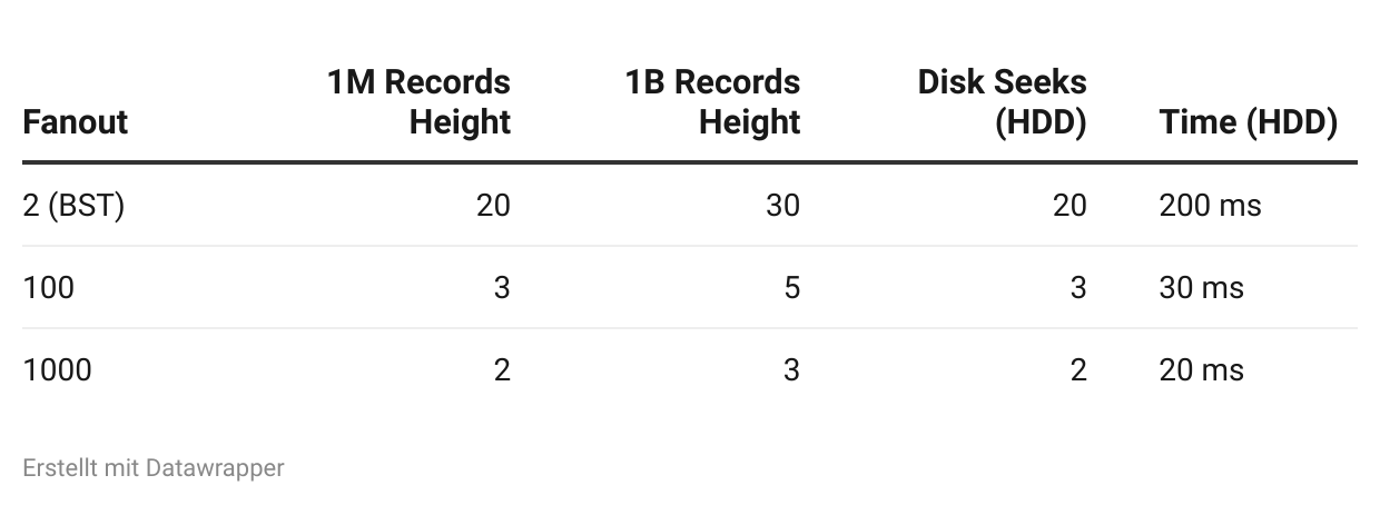
High fanout = fewer disk seeks = faster queries.
B-Tree Lookup Algorithm
Finding a key in a B-Tree is a root-to-leaf traversal with binary search at each node.
Algorithm:
Start at the root node
Binary search the keys in the current node to find the separator key range
Follow the corresponding child pointer
Repeat until reaching a leaf node
In the leaf, either find the key or conclude it doesn’t exist
Time complexity:
Tree height: O(log_fanout n)
Binary search per node: O(log₂ fanout)
Total: O(log n)
Example: Find key 72 in a B-Tree with fanout 100 and 1 million records.
Step 1: Read root node (1 disk I/O)
  Keys: [50, 100, 150, ...]
  72 is between 50 and 100
  Follow child pointer 2

Step 2: Read internal node (1 disk I/O)
  Keys: [55, 60, 65, 70, 75, 80, ...]
  72 is between 70 and 75
  Follow child pointer 5

Step 3: Read leaf node (1 disk I/O)
  Keys: [71, 72, 73, 74]
  Found! Return value for key 72

Total: 3 disk I/O operations = 30 ms on HDD, 0.3 ms on SSD
Working Implementation in Python
Let’s implement a simplified but functional B-Tree in Python.
from typing import List, Optional, Tuple
from dataclasses import dataclass, field


@dataclass
class BTreeNode:
    “”“
    B-Tree node storing keys and child pointers.

    Attributes:
        keys: Sorted list of keys in this node
        children: List of child node pointers (len = len(keys) + 1)
        is_leaf: True if this is a leaf node (no children)

    Invariants:
        - len(children) == len(keys) + 1 (for internal nodes)
        - All keys are sorted
        - Keys in children[i] < keys[i] < keys in children[i+1]
    “”“
    keys: List[int] = field(default_factory=list)
    children: List[’BTreeNode’] = field(default_factory=list)
    is_leaf: bool = True

    def __repr__(self):
        return f”BTreeNode(keys={self.keys}, is_leaf={self.is_leaf})”


class BTree:
    “”“
    B-Tree implementation with configurable order.

    Attributes:
        order: Maximum number of children per node (fanout)
        root: Root node of the tree

    Properties:
        - Each node has at most (order - 1) keys
        - Each non-root node has at least (order // 2 - 1) keys
        - Tree height is O(log_order n)

    Time Complexity:
        - Search: O(log n)
        - Insert: O(log n)
        - Delete: O(log n)

    Space Complexity: O(n)
    “”“

    def __init__(self, order: int = 100):
        “”“
        Initialize B-Tree.

        Args:
            order: Maximum number of children per node (fanout).
                   Higher order = fewer levels but larger nodes.
                   Typical values: 100-1000 for disk-based storage.
        “”“
        if order < 3:
            raise ValueError(”Order must be at least 3”)

        self.order = order
        self.root = BTreeNode()

    def search(self, key: int) -> Optional[int]:
        “”“
        Search for a key in the B-Tree.

        Args:
            key: The key to search for

        Returns:
            The key if found, None otherwise

        Time Complexity: O(log n) where n is number of keys
        “”“
        return self._search_recursive(self.root, key)

    def _search_recursive(self, node: BTreeNode, key: int) -> Optional[int]:
        “”“
        Recursively search for key starting from node.

        Uses binary search within each node to find the correct child.
        “”“
        # Binary search within this node
        i = self._binary_search(node.keys, key)

        # Found exact match
        if i < len(node.keys) and node.keys[i] == key:
            return key

        # Reached leaf without finding key
        if node.is_leaf:
            return None

        # Recurse into appropriate child
        # (In real implementation, this would be a disk I/O)
        return self._search_recursive(node.children[i], key)

    def _binary_search(self, keys: List[int], key: int) -> int:
        “”“
        Binary search to find insertion point for key.

        Returns:
            Index i where keys[i-1] < key <= keys[i]

        Time Complexity: O(log m) where m is number of keys in node
        “”“
        left, right = 0, len(keys)
        while left < right:
            mid = (left + right) // 2
            if keys[mid] < key:
                left = mid + 1
            else:
                right = mid
        return left

    def insert(self, key: int):
        “”“
        Insert a key into the B-Tree.

        Args:
            key: The key to insert

        Time Complexity: O(log n)

        Algorithm:
            1. Find the appropriate leaf node
            2. Insert key into leaf
            3. If leaf overflows (too many keys), split it
            4. Propagate split up the tree if necessary
        “”“
        root = self.root

        # If root is full, split it and create new root
        if len(root.keys) >= self.order - 1:
            new_root = BTreeNode(is_leaf=False)
            new_root.children.append(self.root)
            self._split_child(new_root, 0)
            self.root = new_root

        self._insert_non_full(self.root, key)

    def _insert_non_full(self, node: BTreeNode, key: int):
        “”“
        Insert key into a node that is not full.

        Recursively finds the correct leaf and inserts.
        “”“
        i = len(node.keys) - 1

        if node.is_leaf:
            # Insert into sorted position
            node.keys.append(None)  # Make space
            while i >= 0 and key < node.keys[i]:
                node.keys[i + 1] = node.keys[i]
                i -= 1
            node.keys[i + 1] = key
        else:
            # Find child to insert into
            while i >= 0 and key < node.keys[i]:
                i -= 1
            i += 1

            # Split child if it’s full
            if len(node.children[i].keys) >= self.order - 1:
                self._split_child(node, i)
                if key > node.keys[i]:
                    i += 1

            self._insert_non_full(node.children[i], key)

    def _split_child(self, parent: BTreeNode, child_index: int):
        “”“
        Split a full child node into two nodes.

        Args:
            parent: Parent node containing the full child
            child_index: Index of the full child in parent.children

        Algorithm:
            1. Create new sibling node
            2. Move half of keys from full child to sibling
            3. Promote middle key to parent
            4. Update parent’s children list
        “”“
        full_child = parent.children[child_index]
        new_sibling = BTreeNode(is_leaf=full_child.is_leaf)

        mid = (self.order - 1) // 2

        # Move half the keys to new sibling
        new_sibling.keys = full_child.keys[mid + 1:]
        full_child.keys = full_child.keys[:mid]

        # Move half the children if not a leaf
        if not full_child.is_leaf:
            new_sibling.children = full_child.children[mid + 1:]
            full_child.children = full_child.children[:mid + 1]

        # Promote middle key to parent
        promoted_key = full_child.keys[mid] if full_child.is_leaf else full_child.keys[mid]
        parent.keys.insert(child_index, promoted_key)
        parent.children.insert(child_index + 1, new_sibling)

    def print_tree(self, node: Optional[BTreeNode] = None, level: int = 0):
        “”“
        Print tree structure for debugging.
        “”“
        if node is None:
            node = self.root

        print(”  “ * level + f”Level {level}: {node.keys}”)
        if not node.is_leaf:
            for child in node.children:
                self.print_tree(child, level + 1)


# Example usage and demonstration
if __name__ == “__main__”:
    # Create B-Tree with order 5 (max 4 keys per node)
    btree = BTree(order=5)

    # Insert keys
    keys = [10, 20, 5, 6, 12, 30, 7, 17, 3, 16, 21, 24, 25, 26, 27]
    print(”Inserting keys:”, keys)
    for key in keys:
        btree.insert(key)

    print(”\nB-Tree structure:”)
    btree.print_tree()

    # Search for keys
    print(”\nSearching for keys:”)
    for search_key in [6, 16, 21, 100]:
        result = btree.search(search_key)
        if result:
            print(f”  Key {search_key}: FOUND”)
        else:
            print(f”  Key {search_key}: NOT FOUND”)

    # Demonstrate disk I/O count
    print(”\n--- Performance Analysis ---”)
    print(f”Tree order (fanout): {btree.order}”)
    print(f”Max keys per node: {btree.order - 1}”)

    # Estimate tree height for large datasets
    def estimate_height(num_records: int, fanout: int) -> int:
        “”“Estimate tree height for given number of records and fanout.”“”
        import math
        return math.ceil(math.log(num_records, fanout))

    datasets = [
        (”1 thousand”, 1_000),
        (”1 million”, 1_000_000),
        (”1 billion”, 1_000_000_000),
    ]

    fanouts = [5, 100, 1000]

    print(”\nEstimated tree height (= disk seeks):”)
    print(f”{’Dataset’:<15} {’Fanout=5’:<10} {’Fanout=100’:<12} {’Fanout=1000’:<12}”)
    for name, size in datasets:
        heights = [estimate_height(size, f) for f in fanouts]
        print(f”{name:<15} {heights[0]:<10} {heights[1]:<12} {heights[2]:<12}”)

    print(”\nDisk access time on HDD (10ms per seek):”)
    print(f”{’Dataset’:<15} {’Fanout=5’:<10} {’Fanout=100’:<12} {’Fanout=1000’:<12}”)
    for name, size in datasets:
        times = [f”{estimate_height(size, f) * 10}ms” for f in fanouts]
        print(f”{name:<15} {times[0]:<10} {times[1]:<12} {times[2]:<12}”)
Output:
Inserting keys: [10, 20, 5, 6, 12, 30, 7, 17, 3, 16, 21, 24, 25, 26, 27]

B-Tree structure:
Level 0: [12, 20, 25]
  Level 1: [3, 5, 6, 7, 10]
  Level 1: [16, 17]
  Level 1: [21, 24]
  Level 1: [26, 27, 30]

Searching for keys:
  Key 6: FOUND
  Key 16: FOUND
  Key 21: FOUND
  Key 100: NOT FOUND

--- Performance Analysis ---
Tree order (fanout): 5
Max keys per node: 4

Estimated tree height (= disk seeks):
Dataset         Fanout=5   Fanout=100   Fanout=1000
1 thousand      5          2            1
1 million       9          3            2
1 billion       13         5            3

Disk access time on HDD (10ms per seek):
Dataset         Fanout=5   Fanout=100   Fanout=1000
1 thousand      50ms       20ms         10ms
1 million       90ms       30ms         20ms
1 billion       130ms      50ms         30ms
Why this implementation works:
Each node stores up to
order - 1keysSplit operation maintains the B-Tree invariants
Binary search within nodes reduces comparisons
Tree height stays logarithmic
B-Tree Node Splits
When you insert a key into a full leaf node, the node must split.
Split algorithm:
Find the midpoint of the full node
Create a new sibling node
Move half the keys to the new node
Promote the middle key to the parent
If parent is full, split it recursively
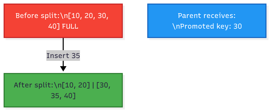
Figure 3: Node split during insertion. The full node is split at the midpoint, and the middle key (30) is promoted to the parent.
When splits propagate to the root:
The root is split into two nodes
A new root is created with one key (the promoted key from the old root)
Tree height increases by 1
This is the only way tree height increases in a B-Tree. B-Trees grow upward from the leaves, not downward from the root.
B-Tree Node Merges
When you delete a key from a node and it becomes too empty (below 50% capacity), it merges with a sibling.
Merge algorithm:
Copy all keys from right sibling to left sibling
Demote the separator key from parent into the merged node
Remove the right sibling
If parent becomes too empty, merge it recursively
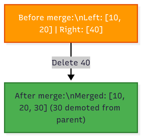
Figure 4: Node merge during deletion. When the right node becomes too empty, it merges with the left node, pulling the separator key from the parent.
When merges propagate to the root:
If the root has only one child after a merge, that child becomes the new root
Tree height decreases by 1
Splits and merges keep the tree balanced. All leaf nodes remain at the same depth, ensuring consistent query performance.
B-Tree Performance Characteristics
Lookup Complexity
Time complexity: O(log n)
For a tree with n keys and fanout f:
Tree height: log_f(n)
Binary search per node: log₂(f)
Total comparisons: log_f(n) × log₂(f) = O(log n)
Disk I/O: log_f(n) disk reads (one per level)
Insert Complexity
Time complexity: O(log n)
Lookup to find insertion point: O(log n)
Insert into leaf: O(f) to shift keys
Split if necessary: O(f) to move keys
Splits propagate up: O(log n) levels in worst case
Disk I/O: O(log n) disk reads + O(log n) disk writes
Delete Complexity
Time complexity: O(log n)
Lookup to find key: O(log n)
Delete from leaf: O(f) to shift keys
Merge if necessary: O(f) to move keys
Merges propagate up: O(log n) levels in worst case
Disk I/O: O(log n) disk reads + O(log n) disk writes
Space Complexity
Space: O(n)
Each key is stored once. Internal nodes add overhead (pointers and separator keys), but this is typically 10-20% of data size.
Occupancy: Nodes are typically 50-90% full. Higher fanout improves space efficiency because pointer overhead becomes proportionally smaller.
Real-World B-Tree Usage
Every major database uses B-Trees (or B+-Trees) for indexes.
MySQL InnoDB
InnoDB uses B+-Trees for:
Primary key index (clustered index): Stores actual row data in leaf nodes
Secondary indexes: Store pointers to primary key in leaf nodes
InnoDB B-Tree configuration:
Page size: 16 KB (default)
Fanout: ~100-200 depending on key size
Tree height for 1 million rows: 3-4 levels
Example:
-- Create table with primary key
CREATE TABLE users (
    id INT PRIMARY KEY,
    name VARCHAR(100),
    email VARCHAR(100)
) ENGINE=InnoDB;

-- Primary key automatically creates a clustered B+-Tree index
-- Leaf nodes contain the actual row data
-- Tree structure: id=1 stored with name and email in leaf

-- Create secondary index on email
CREATE INDEX idx_email ON users(email);

-- Secondary index is a separate B+-Tree
-- Leaf nodes contain email → id mappings
-- To fetch full row: lookup email in idx_email → get id → lookup id in primary key
InnoDB query performance:
-- Fast: Uses B-Tree index
SELECT * FROM users WHERE id = 12345;
-- Disk I/O: 3-4 reads (tree height)

-- Slow: Full table scan
SELECT * FROM users WHERE name = ‘Alice’;
-- Disk I/O: 10,000+ reads (scan all pages)

-- Fast: Uses secondary index
SELECT * FROM users WHERE email = ‘alice@example.com’;
-- Disk I/O: 6-8 reads (3-4 for idx_email + 3-4 for primary key)
PostgreSQL
PostgreSQL uses B-Trees as the default index type.
PostgreSQL B-Tree configuration:
Page size: 8 KB (default)
Fanout: ~50-100 depending on key size
Supports multiple index types (B-Tree, Hash, GiST, GIN, BRIN), but B-Tree is default
Example:
-- Default index is B-Tree
CREATE INDEX idx_user_id ON users(id);

-- Explicitly specify B-Tree
CREATE INDEX idx_user_email ON users USING BTREE(email);

-- View index structure
SELECT * FROM pg_indexes WHERE tablename = ‘users’;
SQLite
SQLite uses B-Trees for both tables and indexes.
SQLite B-Tree configuration:
Page size: 4 KB (default, configurable to 64 KB)
Fanout: ~50-100
All data is stored in B-Trees (no separate heap storage)
Interesting fact: SQLite calls its B-Tree implementation “r-tree” for historical reasons, but it’s actually a B+-Tree.
MongoDB WiredTiger
MongoDB’s WiredTiger storage engine uses B-Trees for indexes.
WiredTiger B-Tree configuration:
Internal page size: 4 KB (default)
Leaf page size: 32 KB (default)
Fanout: ~100-200
Supports prefix compression to increase fanout
Example:
// MongoDB creates B-Tree index on _id by default
db.users.insertOne({ _id: 1, name: “Alice”, email: “alice@example.com” });

// Create secondary index (B-Tree)
db.users.createIndex({ email: 1 });

// Query uses B-Tree index
db.users.find({ email: “alice@example.com” });
// Disk I/O: 3-4 reads (tree height)

// Explain shows index usage
db.users.find({ email: “alice@example.com” }).explain();
// Output: “indexName”: “email_1”, “stage”: “IXSCAN”
Trade-offs and Limitations
B-Trees are not perfect. Here’s when they struggle:
1. Write Amplification
Every insert may trigger splits all the way to the root. In the worst case:
Insert 1 key → split leaf → split parent → split grandparent → split root
One logical write becomes 4+ physical writes
Example: Inserting 1 million keys with frequent splits:
Logical writes: 1 million
Physical writes (with splits): 2-3 million
Write amplification: 2-3x
Alternative: LSM-Trees (Log-Structured Merge Trees) used by RocksDB, Cassandra, and LevelDB. LSM-Trees batch writes in memory and flush sequentially to disk, avoiding in-place updates.
2. Range Queries on Non-Sequential Keys
B-Trees are optimized for range queries on the indexed key, but struggle with multi-column range queries.
Example:
-- Fast: Range query on indexed column
SELECT * FROM orders WHERE order_date BETWEEN ‘2024-01-01’ AND ‘2024-12-31’;
-- B-Tree traverses leaf nodes sequentially (leaf nodes are linked)

-- Slow: Range query on non-indexed column
SELECT * FROM orders WHERE total_amount BETWEEN 100 AND 200;
-- Must scan entire table (no index on total_amount)

-- Slow: Multi-column range query
CREATE INDEX idx_date_amount ON orders(order_date, total_amount);
SELECT * FROM orders WHERE order_date > ‘2024-01-01’ AND total_amount > 100;
-- B-Tree can use order_date range, but must filter total_amount in memory
Alternative: Multi-dimensional indexes like R-Trees (for spatial data) or hybrid indexes.
3. Memory Overhead for Caching
To avoid disk I/O, databases cache frequently accessed B-Tree nodes in memory. For a large database:
1 billion records
Tree height: 4 levels
Internal nodes: ~1 million
Cache size: ~16 GB (to cache all internal nodes)
Rule of thumb: Plan for 10-20% of your database size in RAM for B-Tree caches.
4. Fragmentation Over Time
After many inserts and deletes, B-Tree nodes may be only 50-60% full. This wastes space and increases tree height.
Solution: Periodic VACUUM (PostgreSQL) or OPTIMIZE TABLE (MySQL) to rebuild B-Trees.
Example:
-- PostgreSQL: Rebuild table and indexes
VACUUM FULL users;

-- MySQL: Optimize table (rebuilds B-Tree)
OPTIMIZE TABLE users;
5. Concurrency Challenges
B-Trees require locking during splits and merges. In high-concurrency workloads, lock contention can bottleneck writes.
Solution: Latch-free B-Trees (used in modern databases like Microsoft SQL Server) or MVCC (Multi-Version Concurrency Control).
When NOT to Use B-Trees
B-Trees are excellent for disk-based sorted data, but not always optimal:
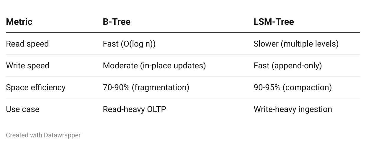
Write-Heavy Workloads
If you’re doing 100,000 writes/sec with few reads, LSM-Trees outperform B-Trees.
Comparison:
Examples:
B-Tree: MySQL, PostgreSQL, SQLite
LSM-Tree: RocksDB, Cassandra, LevelDB
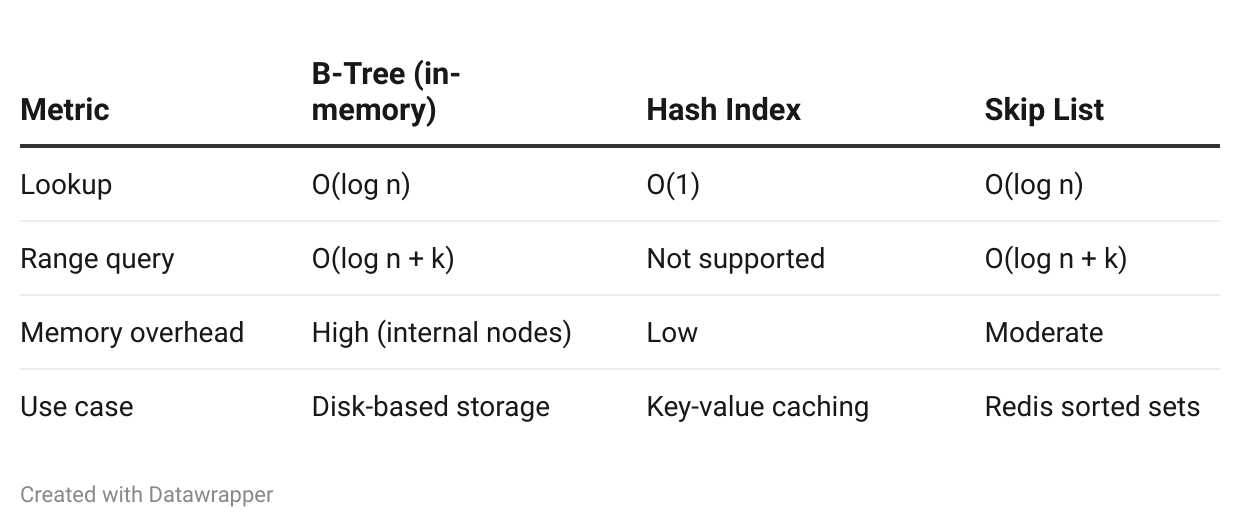
In-Memory Databases
If your entire dataset fits in RAM, B-Trees add unnecessary complexity. Hash indexes or skip lists are simpler and faster.
Comparison:
Examples:
Hash index: Memcached, Redis hashes
Skip list: Redis sorted sets
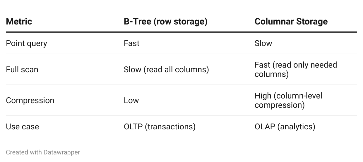
Analytical Workloads (OLAP)
For large analytical queries scanning millions of rows, columnar storage (e.g., Parquet, ORC) outperforms B-Trees.
Comparison:
Examples:
Row storage (B-Tree): MySQL, PostgreSQL
Columnar storage: Parquet (used by Snowflake, BigQuery), ORC (used by Hive)
Summary: Why B-Trees Won
After 50+ years, B-Trees remain the dominant on-disk data structure because they:
Minimize disk I/O: High fanout reduces tree height
Balance automatically: Splits and merges keep all leaves at the same depth
Support range queries: Sorted keys and leaf-level links enable efficient scans
Work on any disk: Optimized for both HDDs (sequential I/O) and SSDs (block-level access)
Key insight: B-Trees match the constraints of disk storage. Since the smallest I/O unit is a block, B-Trees pack as much data as possible into each block. This simple idea—maximizing fanout to minimize height—makes databases fast.
When to use B-Trees:
Disk-based storage (database indexes)
Frequent reads and moderate writes
Range queries on sorted data
General-purpose OLTP workloads
When to consider alternatives:
Write-heavy workloads (LSM-Trees)
In-memory data (hash indexes, skip lists)
Analytical queries (columnar storage)
Every time you query your database and get a result in milliseconds, thank the B-Tree.
References
This article is based on Chapter 2 (”B-Tree Basics”) of Database Internals: A Deep Dive into How Distributed Data Systems Work by Alex Petrov (O’Reilly, 2019).
Additional resources:
Bayer, R., & McCreight, E. (1972). “Organization and Maintenance of Large Ordered Indexes.” Acta Informatica, 1(3), 173-189. https://doi.org/10.1007/BF00288683
Comer, D. (1979). “The Ubiquitous B-Tree.” ACM Computing Surveys, 11(2), 121-137. https://doi.org/10.1145/356770.356776
Graefe, G. (2011). “Modern B-Tree Techniques.” Foundations and Trends in Databases, 3(4), 203-402. https://doi.org/10.1561/1900000028
MySQL Documentation: “InnoDB B-Tree Indexes” https://dev.mysql.com/doc/refman/8.0/en/innodb-physical-structure.html
PostgreSQL Documentation: “B-Tree Indexes” https://www.postgresql.org/docs/current/btree.html
SQLite Documentation: “B-Tree Module” https://www.sqlite.org/btreemodule.html
Books:
Petrov, A. (2019). Database Internals: A Deep Dive into How Distributed Data Systems Work. O’Reilly Media. ISBN: 978-1492040347
Knuth, D. E. (1998). The Art of Computer Programming, Volume 3: Sorting and Searching (2nd Ed.). Addison-Wesley. ISBN: 978-0201896855
Graefe, G. (2011). Modern B-Tree Techniques. Now Publishers. ISBN: 978-1601984197
Thanks for reading!
If you found this deep-dive helpful, subscribe to m3mo Bytes for more technical explorations of databases, distributed systems, and data structures.
Have you worked with B-Trees or database indexes? What performance challenges have you faced? Share your experiences in the comments—I read and respond to every one.
Discussion
What database systems have you worked with? (MySQL, PostgreSQL, MongoDB?)
Have you encountered B-Tree performance bottlenecks in production?
What index strategies have worked well for your workload?
Have you compared B-Trees to LSM-Trees for write-heavy workloads?
Any interesting query optimization stories with indexes?
Drop a comment below.